Section 7: match() and optional()

Suppose you have this graph: two A-B-C paths share a common B node, and B is also connected to X and Y nodes.

You want to find only the C nodes that are connected via a B node that also has X→Y connections. You want C2, not C1.

A single traversal cannot express this. You would have to walk the entire path A→B→C→…​→X→Y, which may not be structurally possible, or run two separate queries and intersect the results in your script.

match() solves this directly.

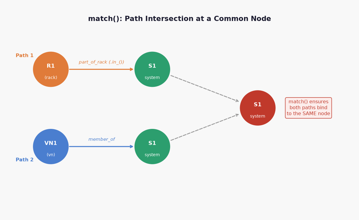
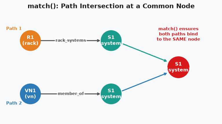
match() takes two or more complete traversal expressions, separated by commas, and returns only the result rows where all traversals are simultaneously satisfiable.

The critical element is the shared name=: both traversals reference name='b'. The query engine finds rows where the same physical node satisfies the B position in the first traversal and the middle position in the second traversal. Rows where that node is different in each traversal are excluded.

This is the graph query equivalent of an inner join on a shared value.

In the second traversal within the match(), notice that the middle node is written as just node(name='b') — with no type filter.

When a node already has a name= binding from an earlier traversal in the same match(), you do not need to re-specify its type. The engine already knows exactly which node b is — it was resolved in the first traversal. Repeating the type would be redundant. What matters is that the second traversal also finds a valid path through that already-identified node.

When would you use match()? The clearest real-world scenario: finding virtual networks whose routing zone also has a routing policy attached.

This is the DC - Virtual Networks with their routing policies predefined catalog query. It is a single chained traversal, not a multi-path intersection, but it demonstrates how match() wraps a complete traversal. The wrapper is necessary when using optional() alongside it, which you will see in the next section.

The DC - All fabric interfaces query combines two traversals to find only leaf/spine links that have a confirmed remote system:

This single match() traversal walks the complete link path and names five nodes — system, iface, link, remote_iface, remote_system — all in a single result row. Every result is a fully qualified link from a deployed leaf or spine to a deployed spine, access, or superspine.

When you write a traversal A.out().B.out().C, every result must contain A, B, and C. If C does not exist for a given A-B pair, that pair is excluded entirely.

But sometimes you want: "find all A-B pairs, and if C also exists, include it — but don’t drop A-B pairs just because C isn’t there".

That is optional().

A server can be connected to the fabric in three ways:

In the graph, a single-homed server connection looks like:

system → interface → link → interface → system

A LAG-homed connection adds two levels of abstraction:

system → interface(AE) → interface → link → interface(AE) → system

An ESI-homed connection adds a redundancy_group node as well.

If you write a traversal that assumes the full ESI path, you will miss all single-homed and LAG-homed connections. optional() lets you find the base path and capture the extra nodes if they exist.

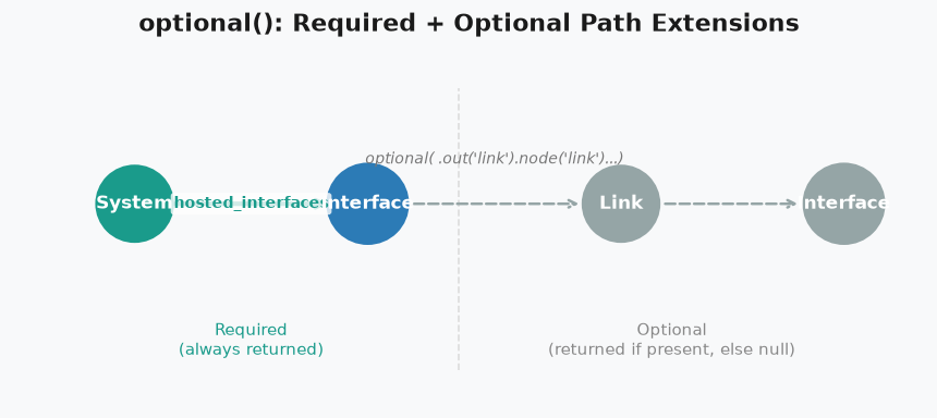
The optional() block starts from a named node that was already found in the required traversal (name='t1'). It tries to extend the path from that node. If the extension exists, the result includes t2. If it does not exist, the result still includes t1 — it is not dropped.

Optional blocks can be nested to handle multiple levels of conditional depth:

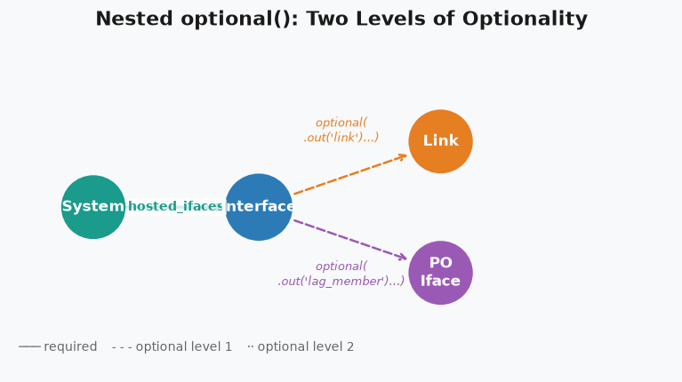
This reads:

In the API response, a result for a simple connection contains only t1. A result for a LAG connection contains t1 and t2. A result for an ESI connection contains t1, t2, and t3.

When would you use nested optional? The ESI link discovery use case above is the canonical example. You are walking the connection topology of servers in the fabric and need to handle all three attachment types in a single query, producing a result that tells you which type each server uses.